Compute exponential growth from SPARK3D

This script showcases how the exponential growth factor from a bunch of SPARK3D simulations can be calculated. The original data can be manually exported from SPARK3D, or automatically generated (command line SPARK3D).

Pre-requisites

Import some objects:

from pathlib import Path

import numpy as np

from simultipac.simulation_results.simulations_results import (
    SimulationsResults,
    SimulationsResultsFactory,
)

[INFO    ] [log_manager.py      ] Starting log for Simultipac - Version: 2.0.1.dev22+g1f37471.d20250203, Commit: 28c1c760d62f7c4764c2f184225d1fd6853764bb

Loading the data

The factory is used to create the SimulationsResults objects. You will need to provide the RF frequency in GHz.

factory = SimulationsResultsFactory("SPARK3D", freq_ghz=1.30145)

The SimulationsResults object will hold all the data. You must provide:

1. The path to the file holding the results. Check dedicated documentation for the format of the results file.

2. The accelerating fields in V/m.

As for now, it is not possible to provide the RMS power instead of the accelerating field. It is a very straightforward implementation, but I never had the use for it.

results: SimulationsResults = factory.create(
    filepath=Path("../../../examples/spark/time_results.csv"),
    e_acc=np.linspace(1e6, 3e7, 30),
)

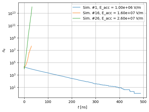
You can visualize the evolution of the population with the SimulationsResults.plot method. Here, we only plot the first, 16th and 26th simulations.

idx_to_plot = (0, 15, 25)
pop_axes = results.plot(x="time", y="population", idx_to_plot=idx_to_plot, alpha=0.7)
pop_axes.set_yscale("log")

Calculating exponential growth factor

The running mean keyword allows to average the evolution of the population over a RF period. It is useless with SPARK3D, as there are only 1 or 2 points per RF period.

results.fit_alpha(fitting_periods=20, running_mean=False)

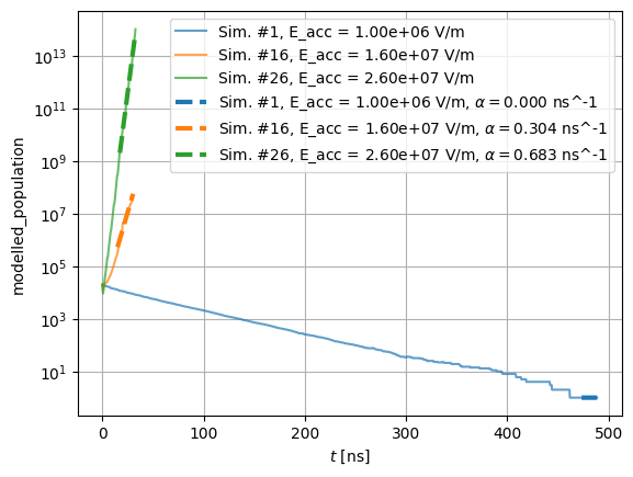
The modelled population can be plotted with:

pop_axes = results.plot(
    x="time",
    y="modelled_population",
    idx_to_plot=idx_to_plot,
    axes=pop_axes,
    lw=3,
    ls="--",
)
# Trick to force display of figure
fig = pop_axes.get_figure()
fig

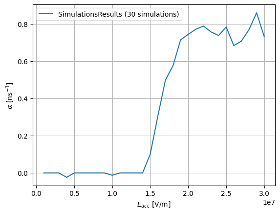
You can also plot the evolution of the exponential growth factor with:

alpha_axes = results.plot(x="e_acc", y="alpha")