Compute exponential growth from CST

This script showcases how the exponential growth factor from a bunch of CST simulations can be calculated.

Pre-requisites

Import some objects:

from pathlib import Path

import numpy as np

from simultipac.simulation_results.simulations_results import (
    SimulationsResults,
    SimulationsResultsFactory,
)

[INFO    ] [log_manager.py      ] Starting log for Simultipac - Version: 2.0.1rc1.dev1+ga19711d.d20250408, Commit: f43dd67ceb1c7530f77719dbdd2b3b515d921c0f

Loading the data

The factory is used to create the SimulationsResults objects. You will need to provide the RF frequency in GHz.

factory = SimulationsResultsFactory("CST", freq_ghz=1.30145)

[INFO    ] [singleton.py        ] Called __call__ (None)

The SimulationsResults object will hold all the data. You must provide:

1. The path to the folder holding the results. Check dedicated documentation for the format of the results folder.

results: SimulationsResults = factory.create(
    master_folder=Path("../../../examples/cst/Export_Parametric"),
)

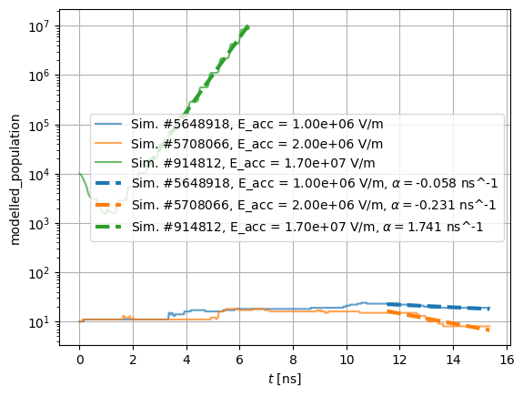
You can visualize the evolution of the population with the SimulationsResults.plot method. Here, we only plot the first, 6th and 91th simulations.

idx_to_plot = (0, 5, 90)
pop_axes = results.plot(x="time", y="population", idx_to_plot=idx_to_plot, alpha=0.7)
pop_axes.set_yscale("log")

Calculating exponential growth factor

The running mean keyword allows to average the evolution of the population over a RF period. It is recommended with CST, as there are many points per RF period.

results.fit_alpha(fitting_periods=5, minimum_final_number_of_electrons=5, running_mean=True)

The modelled population can be plotted with:

pop_axes = results.plot(
    x="time",
    y="modelled_population",
    idx_to_plot=idx_to_plot,
    axes=pop_axes,
    lw=3,
    ls="--",
)
# Trick to force display of previously plotted figure
fig = pop_axes.get_figure()
fig

You can also plot the evolution of the exponential growth factor. Note that there parametric plot are supported; the keys in sort_by_parameter arguments must be present in the mmdd_xxxxxxx/Parameters.txt files.

alpha_axes = results.plot(x="e_acc", y="alpha", sort_by_parameter=("size_cell","N_0"))

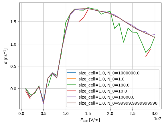
In these simulations, N_0 was the initial number of electrons. Here, N_0 = 1000 appears to be the minimum number for convergence of results.